Inverse Transform Sampling and Maximum Likelihood Estimation

Introduction

In this blog post we are going to look at how we can generate a random sample out of a random variable, and then look at the maximum likelihood method for estimating the parameters of distribution of that random variable.

Generating a random sample

Let's assume we have a sample $x_1,...,x_n$ out of a sequence of i.i.d. random variables $X_1,...,X_n \sim X$, where X for example has Poisson distribution with parameter $\theta$.

How can we generate that random sample in Python by ourselves?

Inverse probability integral transform

We can use discrete Inverse Transform Sampling for generating a Poisson($\theta$) random sample out of an uniformly distributed one. How can we do that?

Given a random variable X, we define a random variable $Y = F_X(X)$ and calculate it's cummulative density function $F_Y(y) = P(Y \le y)$.

From the equation above we see that $Y \in Unif(0, 1)$ and we can generate X by using the fact that $X=F_X^{-1}(Y)$. But what exactly is $F_X^{-1}(Y)$? For example, with $F_X^{-1}(\frac{1}{2})$ we are simply asking the question
$P(X \le ?) = \frac{1}{2}$ i.e. for what value of x we have that $P(X \le x) = \frac{1}{2}$.

In our case X is a discrete random variable which means that $F^{-1}_X(p)=min\{x: F(x)=p, 0 \le p \le 1\}$

But since p is going to intersect a certain rectangle and we are taking discrete values of x, we should take the infimum of x at which $F(X \le x) = p$

Thus, we can just set
$X = 0$, when $Y \le p_X(0)$ and $$ X = k \text{, when } \sum_{i=0}^{k-1}{p_X(i)}< Y \le \sum_{i=0}^k{p_X(i)}, \text{ for } k \ge 1 $$

Let's create a function which generates an outcome out of a Poisson random variable

import math
import random
import matplotlib.pyplot as plt

def inverse_poisson_outcome(theta):
  unif = random.uniform(0, 1)
  probability = math.exp(-theta)
  mass = probability
  k = 0
  while mass < unif:
    k += 1
    probability *= theta / k # since $a^2$
    mass += probability
  return k

And a function which generates an entire sample out of a Poisson random variable

def rpoi(n, theta):
  return [inverse_poisson_outcome(theta) for _ in range(n)]

Estimating the parameters of a random variable

Let's assume we have a Poisson random sample $x_1, ..., x_n \sim X \in Poi(\theta)$ for which we don't know the real parameter $\theta$.

For example we can use the above code to generate a random sample out of a Poisson random variable with parameter $\theta = 10$ and pretend we have no idea what the parameter is.

random.seed(23)
data = rpoi(n=20, theta=10)
> print(data) # [15, 15, 14, 6, 11, 9, 10, 7, 7, 9, 8, 9, 4, 6, 12, 9, 10, 12, 9, 5]

Maximum likelihood estimator

If we look at the probability mass function $$P(X=k; \theta) = p(k;\theta)=\frac{e^{-\theta}\theta^k}{k!}$$ for a fixed parameter $\theta$, we can ask the question 'What is the probability that X equals 14?' $$ P(X_1=14; \theta) = p(14;\theta)=\frac{e^{-\theta}\theta^{14}}{14!} $$ But since the random variables $X_1,...,X_n$ are independent we can ask the question for the entire sample. $$ L(\theta; \textbf{x}) := P(X_1=x_1,...,X_n=x_n ; \theta) = \prod_{i=0}^n{P(X_i=x_i ; \theta)} = \prod_{i=0}^n{\frac{e^{-\theta}\theta^{x_i}}{x_i!}} $$

Writing our log likelihood function in Python would be

  def likelihood(dataset, theta):
    return sum([y*math.log(theta) - theta for y in dataset])
  

We can see that for different values of $\theta$ we still have a joint probability function which as a function of the parameter $\theta$ we call Likelihood function. So, a natural question we can ask is for what value of $\theta$ this likelihood function is maximal? Since we are interested in a maximum of a function, it might be easier to use a monotonic transformation over the likelihood function. The maximum $\hat{\theta}$ for which the function is at maximum is still going to be the same. That estimation $\hat{\theta}$ for $\theta$ is called Maximum likelihood estimation

Plotting the function we get

plt.plot([likelihood(data, th) for th in range(1, 40)])
plt.xlabel('theta parameter')
plt.ylabel('likelihood')
plt.show()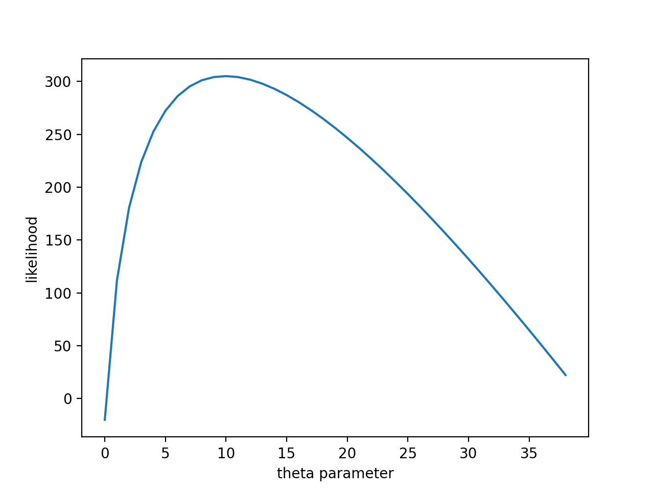

We see that the values $\theta$ for which our sample outcome is more probable i.e. our likelihood function is at it's maximum are around 10, which is the real parameter with which we generated our sample.

Using simple calculus, differentiating our log likelihood function with respect to $\theta$ and setting that derivative to 0, we get

Which gives us

Checking that the second partial derivative is negative does indeed show that for $\hat{\theta}$ the likelihood is at a maximum.

Bisection method

def bisect(dataset, left, right, n, cmp, precision=4):
  for _ in range(n):
    middle = (left + right) / 2
    [left, right] = sorted([left, middle, right], key=cmp)[0:2]
  return round(middle, precision)

Let's dissect our bisect method :) . We simply take two points, include the one in the middle (their average) and repeat the process for the points for which the likelihood is greatest.

> mle = bisect(data, start=5, end=6, n=13, cmp=lambda x: -likelihood(data, x))
> print(mle) # 10.0098

As you can see, our numerical method for estimating the parameter $\theta$ gives a decent approximation for the real value.

Conclusion

I hope you enjoyed this blog post and learned something new. The MLE is a useful estimator having many nice properties like Efficiency, Consistency and Asymptotic Normality